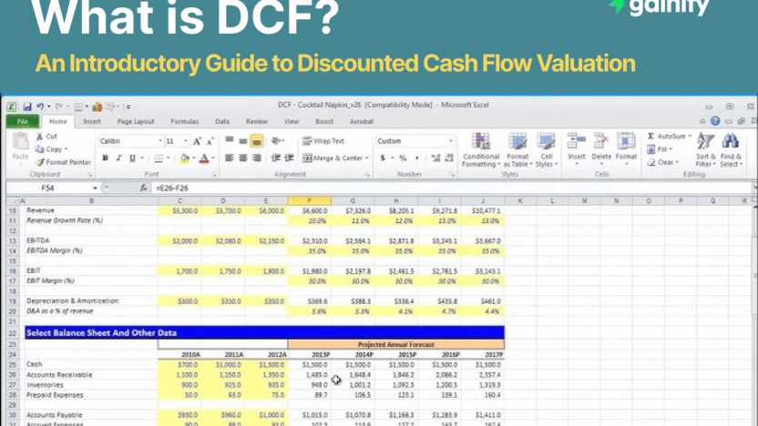

The Discounted Cash Flow (DCF) model is one of the most important tools in finance. It is used to estimate the intrinsic value of an investment by projecting its future cash flows and discounting them back to today’s value.
The principle is straightforward: a dollar received in the future is worth less than a dollar today. Money carries a time value because it can earn interest if invested, and it carries risk because future payments are uncertain. By applying a discount rate that reflects risk and opportunity cost, investors can translate future cash flows into their present value.
When people ask what is DCF, the answer is that it is a valuation method grounded in cash flows rather than accounting profits or market multiples.
It is widely viewed as a gold standard of valuation. At the same time, DCF is highly sensitive to assumptions, which means small changes in inputs such as growth rates or discount rates can significantly alter results. Its greatest strength is that it forces analysts to think carefully about the future, but this also exposes its greatest weakness.
Why DCF Matters
DCF analysis plays a central role across corporate finance, investment banking, and asset management. It is used in:
- Equity research, to determine whether a stock is undervalued or overvalued compared to its trading price.
- Mergers and acquisitions, where buyers and sellers negotiate based on intrinsic worth rather than just comparables.
- Private equity and venture capital, to assess the potential value of portfolio companies.
- Corporate decision-making, such as whether to expand into a new market, invest in new equipment, or pursue an R&D project.
- Project finance and infrastructure, where large-scale projects require cash flow forecasts over decades.
Unlike multiples-based valuation (P/E, EV/EBITDA), DCF does not rely directly on peer comparisons. It instead seeks to answer: “What is this asset worth on its own, given the cash it can generate?”
This makes DCF particularly valuable when comparable companies are scarce, or when a firm’s cash flow profile differs meaningfully from industry averages.
The Core Formula
At its core, the DCF model says:
The value of an asset = the sum of all the money it will make in the future, adjusted back to today’s value.
General DCF Formula
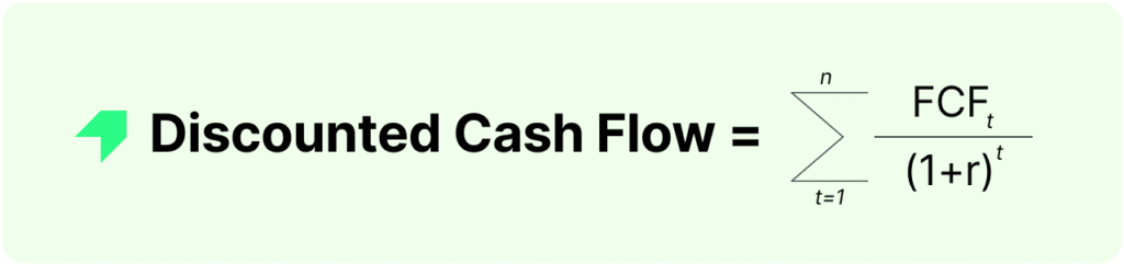
Where:
- FCFₜ = the cash flow expected in year t (for example, profit available to investors)
- r = the discount rate (the return investors require, often based on the company’s cost of capital)
- n = the number of years you are forecasting
How to Think About It
- Imagine a company pays you $100 one year from now. If your required return is 10%, that $100 is only worth about $91 today.
- If it pays $100 five years from now, it is worth even less today, because you have to wait longer.
- The DCF simply adds up all of these “today values” of future payments.
In short: DCF adds up all future cash flows but shrinks them the further away they are, because money today is always worth more than money tomorrow.
Key Components of DCF
1. Forecasting Free Cash Flow (FCF)
The most important input in DCF is free cash flow (FCF), which represents the cash available to all investors (equity and debt holders) after covering operations and reinvestments. Unlike accounting earnings, FCF focuses on actual cash generation.
Free Cash Flow to the Firm (FCFF):

FCF= EBIT×(1−Tax Rate) + Depreciation & Amortization − CAPEX − ΔWorking CapitalFCF
Where:
- EBIT = operating profit (before interest and taxes)
- Depreciation & Amortization = non-cash charges added back
- CAPEX = investments in property, plant, and equipment
- Δ Working Capital = increase or decrease in working capital requirements
This calculation ensures FCF captures the resources left over after a business funds both day-to-day operations and long-term investments. Analysts often prefer FCFF because it reflects the total cash generation available to service all providers of capital.
In practice, projecting FCF requires detailed assumptions about revenue growth, margins, reinvestment needs, and working capital efficiency. This is where sector knowledge and management guidance become critical.
2. The Forecast Period
DCF models generally forecast cash flows for 5–10 years. This period should be long enough to capture the company’s near-term growth and investment cycle, but not so long that projections become speculative.
For mature companies in stable industries, a 5-year forecast may suffice. For younger firms in high-growth sectors, analysts may extend the horizon to 10 years or more. The choice depends on the visibility of cash flows and the company’s competitive position.
Analysts also need to ensure that by the end of the forecast horizon, the business has reached a “steady state” in terms of growth and margins, which makes it reasonable to apply a terminal value.
3. Terminal Value
Because most businesses do not stop operating after 5–10 years, the terminal value (TV) accounts for all the cash flows that come after the forecast horizon. In most DCF models, the terminal value often represents more than half of the total valuation, which makes it a critical part of the analysis.
There are two main ways to calculate it:
A. Perpetuity Growth Method (Gordon Growth Model)
This approach assumes the company will continue generating free cash flows indefinitely, growing at a stable long-term rate.
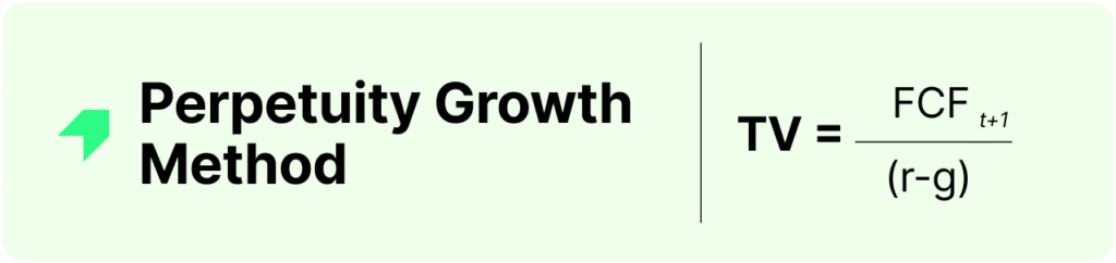
Where:
- FCF₍ₙ₊₁₎ = the free cash flow in the first year after the forecast period
- r = discount rate (required return)
- g = perpetual growth rate of cash flows
👉 In practice, g is usually 2–3%, close to long-term inflation or GDP growth. The idea is that no company can outgrow the overall economy forever.
Example:
If a company is expected to generate $200m in free cash flow after the forecast period, with a discount rate of 8% and a growth rate of 2%, the terminal value is $3333m.
That value is then discounted back to today’s terms.
B. Exit Multiple Method
This method assumes that after the forecast horizon, the company can be sold at a market multiple, similar to how businesses are valued in real-world transactions.
The terminal value is estimated by applying an industry multiple (like EV/EBITDA) to the company’s projected financials in the final forecast year.
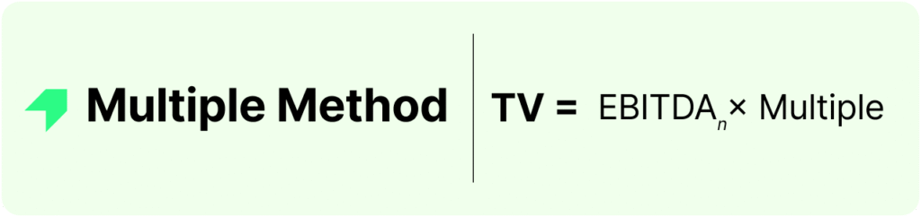
Where:
- EBITDAₙ = earnings before interest, taxes, depreciation, and amortization in the final year of the forecast
- Multiple = an industry-average multiple (based on comparable companies or precedent transactions)
Example:
If a company’s EBITDA in year 5 is $500m and comparable firms trade at 8x EBITDA, then:
TV=500×8=$4,000m
This value is also discounted back to today.
Comparing the Two Methods
- Perpetuity Growth Method is more theoretical, grounded in long-term economics, and widely used in academic and professional valuations.
- Exit Multiple Method is more market-driven, relying on observed multiples in comparable companies or deals.
In practice, analysts often calculate both to cross-check results, since each has its own strengths and limitations.
4. Discount Rate
The discount rate reflects both the time value of money and the riskiness of cash flows. For valuing the entire firm, analysts usually apply the Weighted Average Cost of Capital (WACC):

Where:
- E= market value of equity
- D = market value of debt
- rₙe = cost of equity (often estimated via the Capital Asset Pricing Model (CAPM)
- rₙe = cost of debt, adjusted for taxes
WACC ensures that the discount rate reflects the blended required return of all investors. Firms with high leverage may see their cost of equity rise due to increased risk, even if debt financing appears cheaper.
Putting It All Together
The general valuation formula becomes:

To arrive at equity value, subtract net debt:

This allows direct comparison with a company’s current market capitalization.
Strengths of DCF
✅ Intrinsic framework. Focuses on the asset’s ability to generate cash, not market sentiment.
✅ Flexibility. Can be applied to entire firms, projects, or real estate assets.
✅ Forward-looking. Incorporates long-term growth prospects rather than backward-looking multiples.
✅ Decision-making tool. Useful for testing investment scenarios and sensitivity to assumptions.
Limitations of DCF
❌ Assumption-heavy. Small changes in growth, margins, or discount rates can significantly alter results.
❌ Forecasting challenges. Projecting free cash flows beyond a few years is inherently uncertain.
❌ Terminal value dominance. Often 60–70% of the total valuation comes from TV, making the model vulnerable to terminal assumptions.
❌ Market detachment. Intrinsic values may differ from market prices for extended periods, limiting near-term applicability.
Key Takeaways
- DCF estimates intrinsic value by discounting future free cash flows to the present.
- Inputs matter. Forecasts, discount rate, and terminal value are the most sensitive assumptions.
- Useful across finance. DCF is widely applied in investment banking, equity research, and project evaluation.
- Not flawless. Because results are assumption-driven, DCF should be cross-checked with multiples and precedent transactions.